Physics informed neural networks
Physics informed neural networks
PINNs can provide additional information about how the modeled dynamics should behave that isn’t present when trying to learn the surface function alone. Let’s say you have some complicated function $u(t,x)$, rather than trying to learn the outputs alone we augment the training objective with information about the dynamics of $u$ using partial derivatives. This provides an additional error signal to the deep learning model. Original paper: Physics Informed Neural Networks
\[\begin{array}{l} u_t + u u_x - (0.01/\pi) u_{xx} = 0,\ \ \ x \in [-1,1],\ \ \ t \in [0,1],\newline u(0,x) = -\sin(\pi x),\newline u(t,-1) = u(t,1) = 0. \end{array}\]And define,
\[f := u_t + u u_x - (0.01/\pi) u_{xx} = 0\]We can represent these in TensorFlow as
initializer = tf.keras.initializers.GlorotNormal()

inputs = layers.Input(shape=(2,), dtype=tf.float64)
z = layers.Lambda(lambda X: 2.0*(X - lb)/(ub - lb) - 1.0)(inputs)
z = layers.Dense(20, activation="tanh", kernel_initializer=initializer)(z)
z = layers.Dense(20, activation="tanh", kernel_initializer=initializer)(z)
z = layers.Dense(20, activation="tanh", kernel_initializer=initializer)(z)
z = layers.Dense(20, activation="tanh", kernel_initializer=initializer)(z)
z = layers.Dense(20, activation="tanh", kernel_initializer=initializer)(z)
z = layers.Dense(20, activation="tanh", kernel_initializer=initializer)(z)
outputs = layers.Dense(1, kernel_initializer=initializer)(z)

U_model = tf.keras.Model(inputs=inputs, outputs=outputs)

U_model.summary()
def F_model(x,t):
    t = tf.Variable(t)
    x = tf.Variable(x)
    with tf.GradientTape(persistent=True) as tape:
        u = tf.squeeze(tf.cast(U_model(tf.stack([x,t], 1)), tf.float64))
        u_t = tape.gradient(u,t)
        u_x = tape.gradient(u,x)
        u_xx = tape.gradient(u_x, x)
        f = u_t + u*u_x - (0.01/tf.constant(np.pi, dtype=tf.float64))*u_xx
    return f
Training
The training uses a combined dataset of true $u(t,x)$, boundary points, and solutions to $f(t,x)$ which are evaluated simultaneously, and the total loss is a combination of loss due to $u$ and $f$.
\[\text{Loss} = \text{MSE}_u + \text{MSE}_f\]With this loss, we simply train a neural network taking the gradient of the weights with respect to this combined loss.
def train_step(X_u, u_true, X_f):
    with tf.GradientTape() as tape:

        u_pred = tf.cast(U_model(X_u), tf.float64)
        f = F_model(X_f[:,0], X_f[:,1])

        loss = tf.losses.MeanSquaredError()(u_true, u_pred) + tf.reduce_mean(tf.square(f))
    grads = tape.gradient(loss, U_model.trainable_weights)
    optimizer.apply_gradients(zip(grads, U_model.trainable_weights))
    return loss
Example
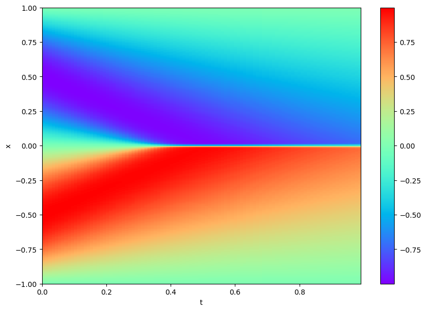
Let’s see an example of PINNs solving a difficult problem using the Burgers’ equation. The notebook for this example can be found here. The expected value of $u(t,x)$ is below. The training set uses 10,000 samples to compute $f(t,x)$ and 50 to compute $u(t,x)$ directly.
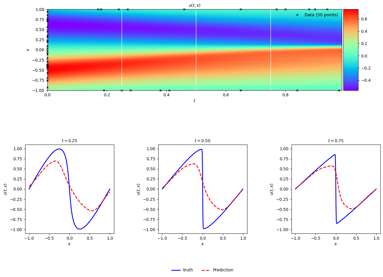
Naïve model
This first example is a neural network with 6 layers of 20 neurons per hidden layer trained without the $f(t,x)$ dataset, simply trying to predict $u(t,x)$. The model is trained using Adam with a learning rate of 0.01, $\beta_1=0.99$ and $\epsilon = 0.1$ for 1000 epochs. The result captures some of the trends in the data but overall performs poorly when tested on the full dataset.
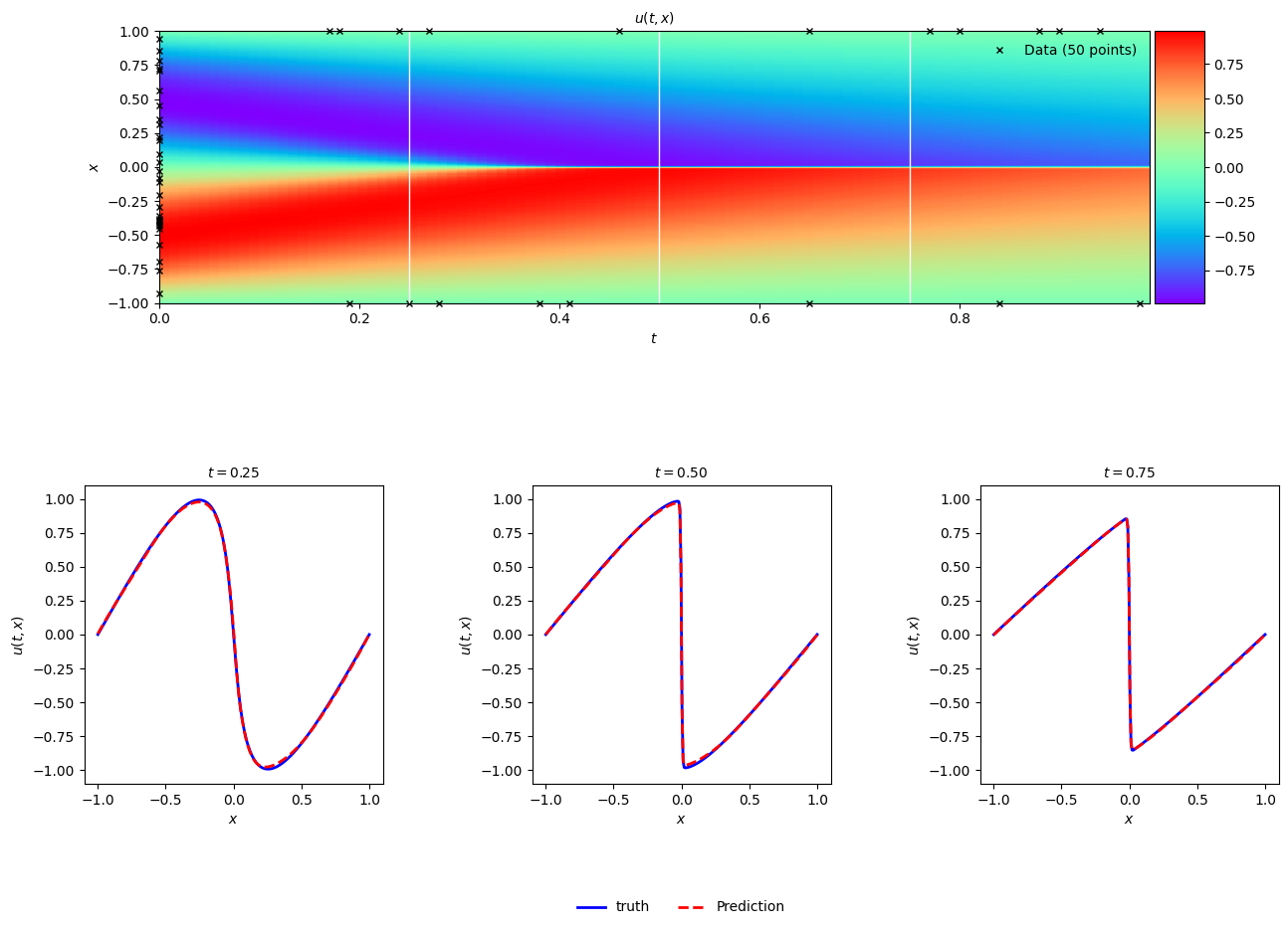
PINN
Now compare this with the same model trained with the partial derivative information and an L-BFGS optimizer replicating the approach used in the paper. The training data in this example comes mostly from the f dataset.
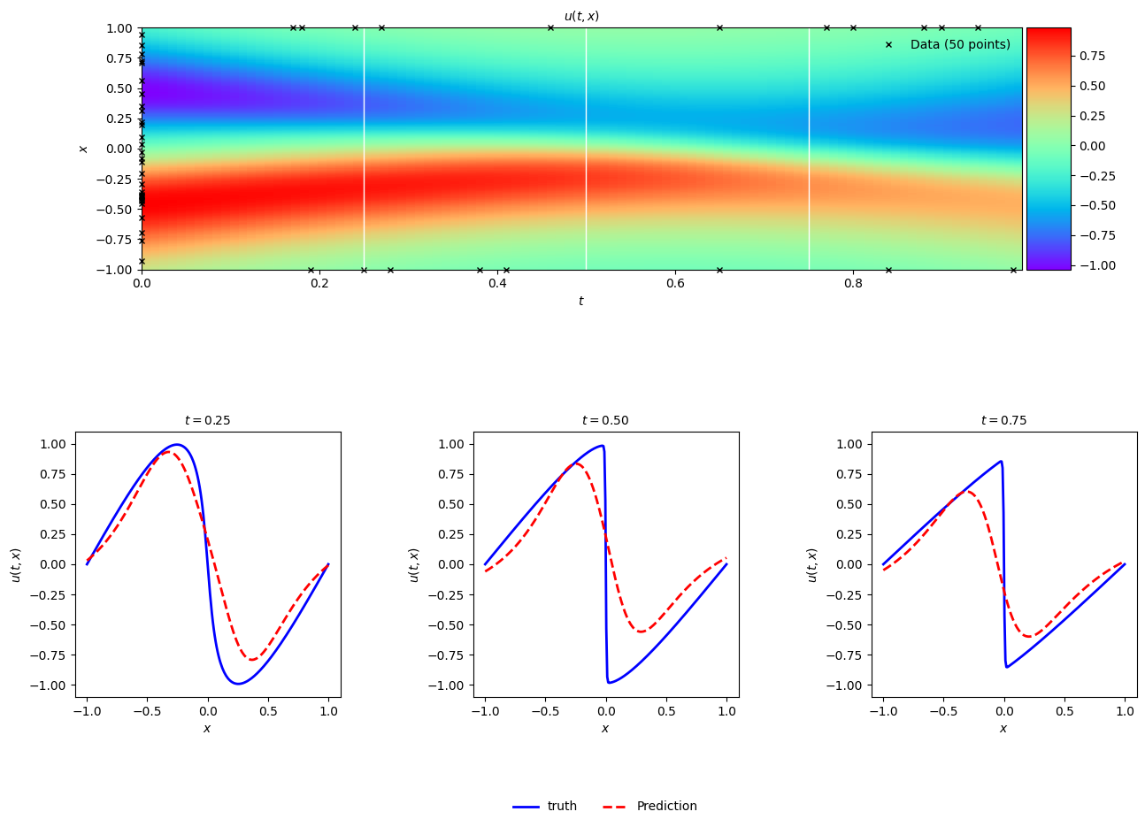
PINN with Adam
This next example uses the same neural network and optimizer as the naïve model, but this time the f dataset with partial derivates is included in the training. While the authors mention training a PINN can be conducted using traditional minibatch methods. This initial stab didn’t work immediately. An L-BFGS approach is likely better with this small dataset, though it can quickly become difficult to compute with more data.