Proximal policy optimization (PPO)
Proximal policy optimization
Proximal policy optimization (PPO) is often described in relation to trust region policy optimization (TRPO). It’s TRPO but better. PPO is an algorithm to deal with common problems in reinforcement learning such as policy instability and large sample sizes.
PPO is an on-policy, actor-critic, policy gradient method that takes the surrogate objective function of TRPO and modifies it into a hard clipped constraint that doesn’t have to be tuned (as much).
Trust region
The trust region is an area around the current objective where an approximation of the true objective is valid. The approximation will diverge from the true objective outside of this region. Taking a step within the trust region will improve the current objective. See this page for a step-by-step illustration of trust-region optimization.
PPO clips the objective function which limits the movement of the parameters, $\theta$, so the difference between the new and old policies remains small. In TRPO, this is implemented using the Kullback-Leibler divergence (KL divergence) as a penalty rather than clipping the importance sampling. Small policy updates within the trust region keep the policy stable during training.
\[L^{C L I P}(\theta)=\hat{\mathbb{E}}_{t}\left[\min \left(r_{t}(\theta) \hat{A}_{t}, \operatorname{clip}\left(r_{t}(\theta), 1-\epsilon, 1+\epsilon\right) \hat{A}_{t}\right)\right]\]where $r_{t}(\theta)=\frac{\pi_{\theta}\left(a_{t} \mid s_{t}\right)}{\pi_{\theta_{\text {old }}}\left(a_{t} \mid s_{t}\right)}$ and $\epsilon$ is a hyperparameter, usually around 0.1 or 0.2
Importance sampling
The ratio $\frac{\pi_{0}\left(a_{t} \mid s_{t}\right)}{\pi_{\theta_{\text {old }}}\left(a_{t} \mid s_{t}\right)}$ is importance sampling weight between the two policies. From Wikipedia:
In statistics, importance sampling is a general technique for estimating properties of a particular distribution, while only having samples generated from a different distribution than the distribution of interest.
Importance sampling has the advantage of being able to compute information about a target distribution with fewer samples than would be required by a Monte-Carlo method and can be used when it’s difficult to sample from the target distribution.
By including the importance sampling weight times the advantage of the sampled policy in the objective function, the agent can learn to reproduce policies that lead to a larger reward.
Entropy
An explanation I’ve heard a lot for entropy is a measure of the disorder in a system. A more useful definition is the average amount of information gained by drawing from a distribution. Unpredictable distributions have higher entropy. This ties into the measure of cross-entropy which measures how close the predicted distribution is to the true one.
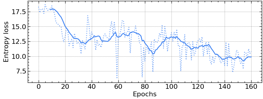
Since this is an on-policy method an additional entropy penalty is added to the loss to increase exploration. Take the entropy of the distributions resulting from evaluating the actor and scale it by a small constant, usually 0.01. This increases the loss for unpredictable distributions. As the actor improves, the entropy of its output distribution decreases.
Algorithm
Run the current policy or $\pi_\text{old}$ with one or many actors in parallel for $T$ steps where $T$ is less than the episode length recording states, actions, rewards, and critic values. Then compute the generalized advantage estimate (GAE), $\hat{A}_t$.
\[\begin{aligned}&\hat{A}_{t}=\delta_{t}+(\gamma \lambda) \delta_{t+1}+\cdots+\cdots+(\gamma \lambda)^{T-t+1} \delta_{T-1} \\&\text { where } \quad \delta_{t}=r_{t}+\gamma V\left(s_{t+1}\right)-V\left(s_{t}\right)\end{aligned}\]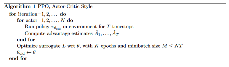 Reproduced from the original paper
Advantage
I’ve seen various implementations of the advantage and loss computation which are not always consistent. Often the advantage computation spans across episode terminations without resetting the reward discounting at the end of an episode. This doesn’t seem to make a difference but is worth looking into further. A TensorFlow implementation is shown below.
def compute_advantages(self, values, next_values, rewards, dones):

        values = tf.cast(values, dtype=tf.float32)

        deltas = np.zeros((len(rewards)))
        for t, (r, v, nv, d) in enumerate(
                zip(rewards, values.numpy(), next_values.numpy(), dones)):
            deltas[t] = r + self.GAMMA * (1 - d) * nv - v

        advantages = copy.deepcopy(deltas)
        for t in reversed(range(len(deltas) - 1)):
            advantages[t] = advantages[t] + (
                1 - dones[t]) * self.GAMMA * self.GAE_LAMBDA * advantages[t + 1]

        targets = advantages + values

        # normalize advantages
        advantages -= tf.reduce_mean(advantages)
        advantages /= (tf.math.reduce_std(advantages) + 1e-8)
        advantages = tf.cast(advantages, dtype=tf.float32)

        return advantages, targets
Loss
Next, compute the surrogate loss using the data collected over $T$ steps using mini-batches for some number of epochs, usually a small number like 3 or 4. Here’s a section of the larger learning function to compute the different losses and update the actor and critic parameters. The actor and critic can share the same bottom layers with different top evaluations or be completely separate networks. The actor network outputs a categorical distribution across the available actions which is used to compute the policy ratio $r_t(\theta)$ and the entropy loss.
for batch in batches:
	with tf.GradientTape() as tape:
	    dist, critic_value, logits = self.agent(states[batch])
	    probs = tf.nn.softmax(logits)

	    action_idx_batch = tf.stack(
	        [tf.range(0, len(probs)), actions[batch]], axis=1)

	    probs = tf.gather_nd(probs, action_idx_batch)

	    critic_value = tf.squeeze(critic_value)

	    entropy = tf.reduce_mean(dist.entropy())

	    # distribution ratio
	    r_theta = tf.math.exp(
	        probs - tf.squeeze(tf.gather(old_probs, batch)))

	    # policy clipping
	    policy_obj = r_theta * tf.gather(advantages, batch)
	    clipped_r_theta = tf.clip_by_value(
	        r_theta, 1 - self.EPS, 1 + self.EPS) * tf.gather(
	            advantages, batch)
	    # compute losses
	    actor_loss = -tf.reduce_mean(
	        tf.minimum(policy_obj, clipped_r_theta))

	    critic_loss = tf.reduce_mean(
	        tf.square(tf.gather(targets, batch) - critic_value))

	    loss = actor_loss + self.C1 * critic_loss + self.C2 * entropy

	    total_loss += loss
	    total_actor_loss += actor_loss
	    total_critic_loss += critic_loss
	    total_entropy_loss += entropy

	grads = tape.gradient(loss, self.agent.trainable_variables)
	self.opt.apply_gradients(
	    zip(grads, self.agent.trainable_variables))
Testing it out
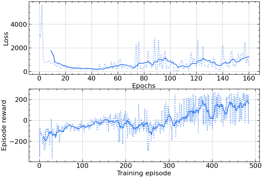
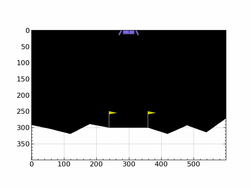
Despite being simpler than TRPO to implement, PPO still requires some tuning of hyperparameters to succeed except in very simple environments. Below are some examples using my TensorFlow implementation on the OpenAI gym discrete lunar lander environment.
Next steps
Now that this discrete version of PPO is working, I want to work on adapting the algorithm for continuous control (testing it on the continuous version of lunar lander) as well as using it on custom environments rather than just the OpenAI gym.
See something wrong or have a question? Contact me or message me on Twitter.