Denoising autoencoders with JAX and Haiku
I previously mentioned the technique of using a denoising autoencoder (DAE) in model-based reinforcement learning (MBRL) to determine when a model was making accurate predictions about the environment (Boney et al. 2019).
A DAE is a fancy name for a model that takes a noisy or corrupted input and attempts to reconstruct the original, uncorrupted data. Typically, this involves an encoder/decoder model where the encoder creates a latent space representation of the input, then the decoder reconstructs the input minus the error signal.
The important idea for MBRL is that the model learns the underlying distribution of the input data during training and can only reconstruct samples that fall inside that distribution. If the trained DAE is presented with input outside this distribution, it won’t successfully reconstruct the original.
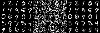
Example original, corrupted and reconstructed data. (source)
The DAE loss can signal when the agent is planning in a familiar region of the state space. If the DAE loss is low, the model can be trusted for planning. If the DAE loss is high, the model is poorly trained in that region so the plan should not be trusted until the region is explored adequately.
From Boney et al. (2019):
The DAE is trained to denoise trajectories that appeared in the past experience and in this way the DAE learns the distribution of the collected trajectories. During trajectory optimization, we use the denoising error of the DAE as a regularization term that is subtracted from the maximized objective function. The intuition is that the denoising error will be large for trajectories that are far from the training distribution, signaling that the dynamics model predictions will be less reliable as it has not been trained on such data.
I had wanted to start exploring JAX (and related packages), the new high-performance library from Google, so this seems like a good time to try it.
JAX and Haiku
JAX is an XLA compiled Python library using a NumPy-like API meaning you can compile and run programs on GPU or TPU extremely quickly as well as use automatic differentiation with Autograd. Haiku is a neural network library built on JAX by DeepMind. JAX has a bit of a learning curve, but it’s a powerful library, and DeepMind moving to it is a strong endorsement.
A significant difference between Haiku and TensorFlow/PyTorch is function transformation. After creating your NN model, you transform it into JAX compatible pure functions mode.init and model.apply. model.init initializes your model with all of the weights to be learned during training and signals what inputs to expect so the model can be compiled appropriately returning the initial model parameters. model.apply takes a set of learned parameters and inputs and returns the model outputs. Here’s an example of transforming and initializing the model, getting the initial parameters back, and using them to initialize the optimizer (using the optimization library for JAX called Optax)
opt = optax.adam(1e-3)

model = hk.without_apply_rng(hk.transform(model_fn))

params = model.init(jax.random.PRNGKey(42),
                    np.random.normal(0,1,(BATCH_SIZE,TIMESTEPS,INPUT_STATE_SIZE)))
opt_state = opt.init(params)
DAE
The objective for the DAE will be to take a corrupted trajectory (set of states and actions) from the Lunar Lander environment and return the real trajectory (set of states). The data is generated by taking random actions in the environment and multiplying each state by a proportional error drawn from a normal distribution with a standard deviation of 20%. Since the action taken determines the next state, the action will be included as input to the DAE but the DAE currently only reconstructs the state history.
Model
The DAE uses two recurrent models as an encoder and decoder to take the noisy input, generate a latent representation, and then decode the uncorrupted trajectory. The full code is here.
class Encoder(hk.RNNCore):
    # note, latent state isn't currently used, instead the final hidden state
    # of the encoder is passed to the decoder
    def __init__(self, hidden_size: int=32, latent_size: int = 64,
                 input_size: int = 8, name=None):
        super().__init__(name=name)
        self._hidden_size = hidden_size
        self._latent_size = latent_size
        self._input_size = input_size

    def initial_state(self, batch_size):
        if batch_size is None:
            shape = (self._hidden_size)
        else:
            shape = (batch_size, self._hidden_size)
        return jnp.zeros(shape)

    def __call__(self, x, state) -> jnp.ndarray:
        x, state = hk.VanillaRNN(self._hidden_size)(x, state)
        return x, state

class Decoder(hk.RNNCore):
    def __init__(self, hidden_size: int=32, latent_size: int = 64,
                 output_size: int = 8, steps :int =20, name=None):
        super().__init__(name=name)
        self._hidden_size = hidden_size
        self._latent_size = latent_size
        self._output_size = output_size
        self._steps = steps

    def initial_state(self, batch_size):
        if batch_size is None:
            shape = (self._hidden_size)
        else:
            shape = (batch_size, self._hidden_size)
        self._batch_size = batch_size
        return jnp.zeros(shape)

    def __call__(self, x, state) -> jnp.ndarray:
        y = jnp.zeros((x.shape[0],self._steps,self._output_size))
        # need to reconstruct trajectory from hidden state,
        # have to loop over RNN since only have first input
        # to start with
        for i in range(self._steps):
            x, state = hk.VanillaRNN(self._hidden_size)(x, state)
            y=y.at[:,i,:].set(hk.Linear(self._output_size)(x))
        return y, state
Haiku has new dynamic and static unroll functions to get the sequence of hidden states and final output from recurrent models. The final encoder state is the decoder initial state.
def model_fn(batch) -> jnp.ndarray:
    # Note: this function is impure; we hk.transform() it below.
    encoder = Encoder(hidden_size=HIDDEN_SIZE, latent_size=LATENT_SIZE,
                      input_size=INPUT_STATE_SIZE)
    decoder = Decoder(hidden_size=HIDDEN_SIZE, latent_size=LATENT_SIZE,
                      output_size=OUTPUT_STATE_SIZE, steps=TIMESTEPS)
    batch_size, sequence_length, _ = batch.shape
    encoder_initial_state = encoder.initial_state(batch_size)

    # output is sequence, state
    _, encoded_state = hk.dynamic_unroll(encoder,
                                        batch,
                                        encoder_initial_state,
                                        time_major=False)

    decoded_sequence, _ = hk.dynamic_unroll(decoder,
                                            jnp.zeros((batch_size, 1, decoder._hidden_size)),
                                            encoded_state, time_major=False)
    return decoded_sequence
The loss function is the MSE between the true trajectory and the model output. The @jax.jit macro compiles everything for fast execution.
@jax.jit
def loss_fn(params: hk.Params, batch) -> jnp.ndarray:
    decoded_sequence = model.apply(params, batch[0])
    return jnp.mean(jnp.square(batch[1] - decoded_sequence))
Training
Updating the parameters with Optax is straightforward and very similar to TensorFlow or PyTorch.
@jax.jit
def update(params: hk.Params, opt_state: optax.OptState, batch) -> Tuple[hk.Params, optax.OptState]:
    grads = jax.grad(loss_fn)(params, batch)
    updates, opt_state = opt.update(grads, opt_state)
    new_params = optax.apply_updates(params, updates)
    return new_params, opt_state
Training the model for 10 epochs before using jit to compile everything took about 2.5 minutes. Adding jit to the loss and update functions sped it up to 14 seconds. It took about 12 seconds to compile, so the actual training took just ~2 seconds!
Results
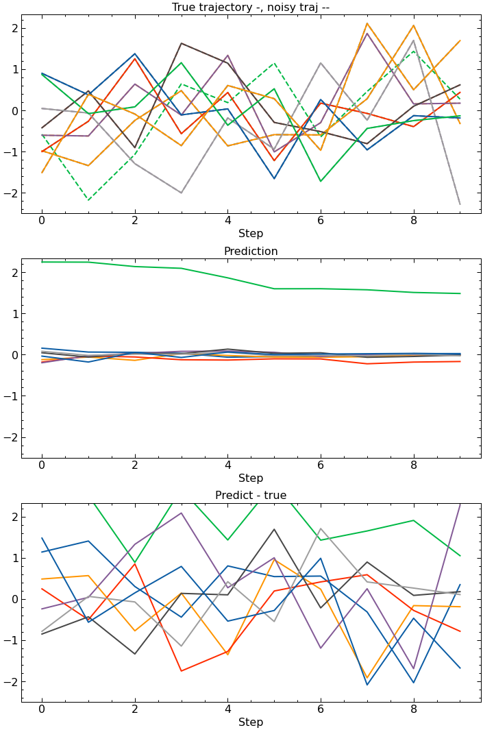
These next couple plots show the true and corrupted trajectory (top), the DAE reconstruction of the true trajectory (middle), and the error between the true trajectory and DAE output. It does pretty well.
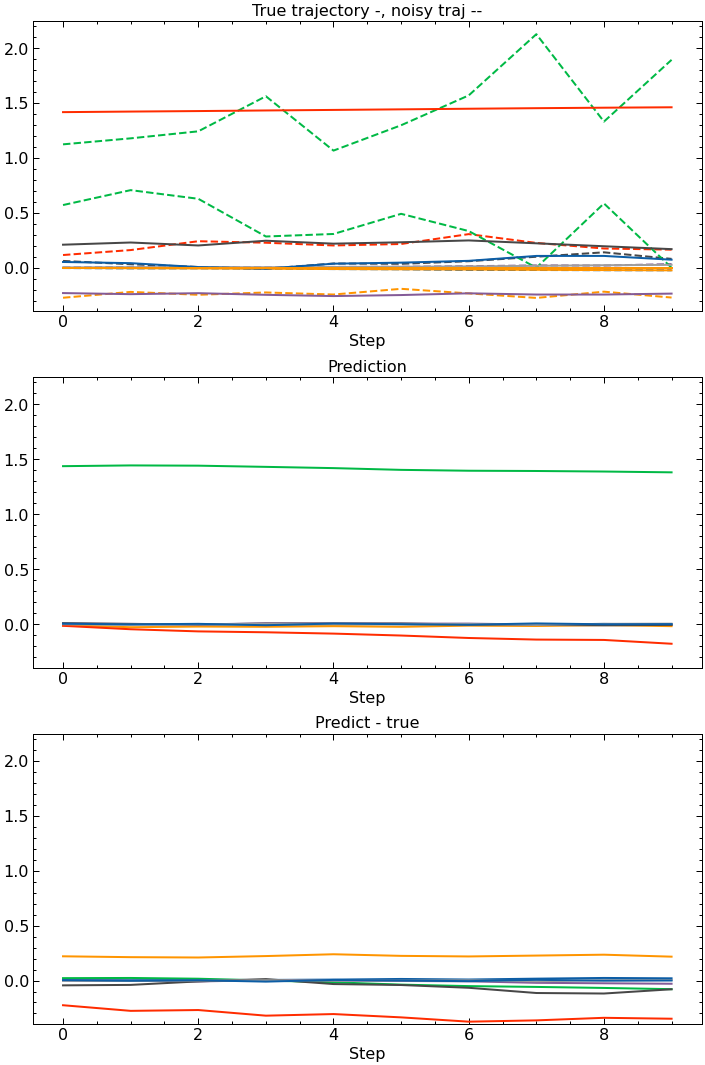
However, if you run the Lunar Lander trained DAE on random noise, representing a poorly trained MBRL environment model, the DAE is unable to reconstruct the input because it doesn’t come from the same distribution as the training data. Now we, hopefully, have a way of knowing how reliable a planned trajectory when training our agent.
References
- Boney, Rinu, Norman Di Palo, Mathias Berglund, Alexander Ilin, Juho Kannala, Antti Rasmus, and Harri Valpola. “Regularizing Trajectory Optimization with Denoising Autoencoders.” ArXiv:1903.11981 [Cs, Stat], December 25, 2019. http://arxiv.org/abs/1903.11981.
- Vincent, Pascal, Hugo Larochelle, Isabelle Lajoie, Yoshua Bengio, and Pierre-Antoine Manzagol. “Stacked Denoising Autoencoders: Learning Useful Representations in a Deep Network with a Local Denoising Criterion.” Journal of Machine Learning Research 11, no. 110 (2010): 3371–3408.